If your bid is late, it loses. In RTB, you often have only 40–50 ms inside the DSP to read signals, score the impression, check budget, and return a price.
So when I think about RTB algorithm design, I keep it simple: use clean data, calibrated prediction, clear automated bid management tools, bid shading for first-price auctions, and hard pacing controls. I also treat testing, privacy checks, and rollback speed as part of the algorithm - not as afterthoughts.
Here’s the short version:
- Latency comes first: every lookup and model call must fit inside a tight time budget.
- Data quality shapes outcomes: use normalized schemas, at least 90 days of history, and keep missing values under 5%.
- Feature choice matters: time-based signals often drive the most lift, so start there.
- Model choice should match the job: logistic regression and GBDT for many CPA/ROAS cases; bandits for low-history traffic; RL only when budget timing effects are large.
- Scores are not bids: convert pCTR/pCVR into bids with calibration, value-per-action logic, and pacing multipliers.
- First-price auctions need shading: bid high enough to win, but not more than needed.
- Guardrails prevent spend drift: use local quotas, caps, fallback rules, and fail-open handling for slow lookups.
- Testing must cover both sides: offline metrics like log-loss and calibration, then live checks for win rate, CPA, ROAS, and spend velocity.
- Privacy and rollout controls belong in-path: consent checks, supply-path validation, canaries, and rollback in under 5 minutes.
That’s the core idea: a strong RTB system is not just a prediction model. It’s a low-latency decision system with tight controls.
Comprehensive Guide to Real-Time Bidding (RTB): Challenges and Opportunities
sbb-itb-89b8f36
Start with Clean Data and Disciplined Feature Inputs
Once the bid optimization goal is set, the next limit is input quality. Before you worry about model choice or bid rules, the data has to be dependable. You need enough history to learn from and enough completeness to trust what the system sees. A good floor is at least 90 days of historical data with less than 5% missing values.
Keep the inputs tight. Capture the fields that shape value, win rate, and pacing:
- auction ID
- timestamp
- placement
- device
- geo
- floor price
- clearing price
- response data
- audience signals
Fix Event Quality Before Adding Model Complexity
The bigger headache is often inconsistent exchange schemas. Supply partners may drift from OpenRTB specs in small but painful ways. So the safest move is to build a normalization layer at ingestion. That layer should convert every payload into one internal canonical format before it touches the feature pipeline or training set.
That step saves you from brittle parser logic later. And in RTB, brittle systems tend to break at the worst time.
There’s another issue: DSPs only see won auctions, which means the training set leans high by default. To correct winner’s-curse bias, use IPS. Log winning bids at 100% and sample losing bids at about 1%.
Choose Features That Reflect Auction Value
Once schema quality is under control, feature selection should follow auction value. The biggest share comes from temporal features at 42%, then audience segments at 27%, contextual signals at 18%, and technical parameters at 13%.
That split tells you where to spend your engineering time first: start with time-based features.
Temporal inputs like hour of day, day of week, and holiday cycles matter because RTB prices can swing hard based on timing. Evening inventory is often the most volatile. A simple and smart way to model this is with sine and cosine time features, which capture cyclical patterns without treating time like a straight line.
Past time signals, other useful inputs include device type, hierarchical geo, publisher category, ad slot position, floor price, placement-level historical CTR/CVR, and conversion lag. Conversion lag is easy to miss, but delayed feedback can throw off bid quality if you ignore it.
And one more thing: feature freshness matters just as much as feature choice. If your signals are stale, even a good model starts making bad calls. Use TTLs of 5 seconds or less on enrichment lookups from in-memory stores. Then use a feature store so training and production stay in sync.
Match the Algorithm to the Bidding Goal
RTB Algorithm Types: Choosing the Right Model for Your Bidding Goal
Clean data and good features help, but they don’t solve everything. You still need an algorithm that fits the bidding goal, the amount of data you have, and how much the auction moves around. Start with the simplest option that can do the job. After that, the next move is turning model scores into bids while staying inside hard budget limits.
Use Simpler Predictive Models When Transparency Matters
Logistic regression and GBDT models like XGBoost or LightGBM are the usual picks for CTR and CVR prediction. They’re easier to debug when things go sideways. That matters when a campaign manager asks why bids fell or why spend jumped, because you can point to the features that pushed the output.
GBDT is better at handling non-linear feature interactions than logistic regression. The tradeoff is speed in production. It often needs deployment work, like compiling to ONNX or C++ if-else trees, to stay inside strict latency budgets. For standard performance campaigns built around CPA or ROAS, these models are often the best place to start.
Use Adaptive Methods When Auction Conditions Shift Quickly
Sometimes the market moves too fast for simpler models. Inventory quality changes. Competition gets tougher. Or you enter a new audience segment with very little history. In those cases, models based only on past averages can lag behind.
That’s where contextual bandits like UCB or Thompson Sampling and reinforcement learning (RL) come in.
Contextual bandits help you balance exploration and exploitation. In plain English, they let you test new traffic, like a new device type or a region with sparse data, without giving up what’s already working. RL goes a step further. It deals with the sequential side of bidding, where a decision now can affect budget left later in the day or week. That makes it a fit for dynamic budget pacing and longer-horizon ROI work.
A simple rule of thumb:
- Use bandits when you need exploration.
- Use RL only when sequential budget effects are big enough to justify the added complexity.
These methods matter most when traffic shifts faster than historical averages.
Map Model Output to Business Metrics
Model choice should tie back to the business goal, not just raw click-through rate. A model tuned only for CTR can win a pile of cheap clicks that never turn into sales. That’s why a standard production scoring function makes the tradeoff plain: Score = Bid × P(click) × P(conversion | click) × Quality Factor.
Each part of that formula should line up with what the campaign is trying to do. If the goal is profit, the score should reflect profit. If the goal is ROAS, the scoring logic should point there too. Otherwise, you can end up optimizing the wrong thing while the dashboard looks fine.
Here’s a quick reference for matching algorithm type to goal:
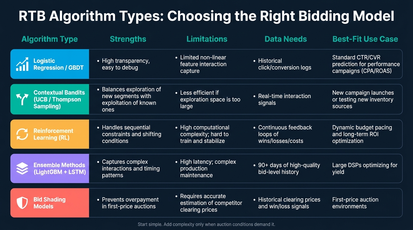
| Algorithm Approach | Strengths | Limitations | Data Needs | Best-Fit Use Case |
|---|---|---|---|---|
| Logistic Regression / GBDT | High transparency, easy to debug | Limited ability to capture complex non-linear feature interactions | Historical click/conversion logs | Standard CTR/CVR prediction for top PPC agencies managing performance campaigns |
| Contextual Bandits (UCB/Thompson Sampling) | Balances exploration of new segments with exploitation of known ones | Can be less efficient if the exploration space is too large | Real-time interaction signals | New campaign launches or testing new inventory sources |
| Reinforcement Learning (RL) | Handles sequential constraints and shifting conditions | High computational complexity; difficult to train and stabilize | Continuous feedback loops of wins/losses/costs | Dynamic budget pacing and long-term ROI optimization |
| Ensemble Methods (LightGBM + LSTM) | Captures complex interactions and timing patterns | High latency; complex production maintenance | 90+ days of high-quality bid-level history | Large DSPs optimizing for yield |
| Bid Shading Models | Prevents overpayment in first-price auctions | Requires accurate estimation of competitor clearing prices | Historical clearing prices and win/loss signals | First-price auction environments |
Even the best score still needs a bid rule, pacing limits, and safety checks.
Convert Model Scores into Bids with Hard Constraints
Once scoring is set, the job shifts to execution: turning value into a bid the auction will accept. That bid still has to fit the messy parts of production, like budget limits, floor prices, and tight latency windows.
Write Bid Formulas That Reflect Expected Value
Start with expected advertiser value, or EAV. A common formula is bid = λ × V × p(conversion), where V is the advertiser’s value per action and λ is a pacing multiplier between 0 and 1. Lower λ, and you become more selective, bidding only on impressions with a better chance of converting.
But there’s a catch. Model scores should be calibrated before they go anywhere near a bid formula. Raw pCTR and pCVR outputs are not true probabilities unless calibration has been done first. If you skip that step, your bid prices drift away from actual value.
In first-price auctions, it also helps to shade bids based on the estimated clearing-price distribution, with the goal of improving expected profit.
After the bid value is chosen, spend control decides how long the campaign can keep using it.
Apply Pacing, Caps, and Safety Checks
Budget pacing is not just a nice idea on a whiteboard. In high-scale systems, strict global budget locks turn into bottlenecks fast. A better setup is local micro-quotas: each node spends from an in-memory sub-budget, then asks for a refill when that bucket runs dry. Most teams also allow a 2% to 5% overspend buffer, because strict global locking is too slow for sub-100 ms bidding.
For smoother spend through the day, PID controllers are a common pick. They update the pacing multiplier by comparing actual spend with the target spend rate, which helps stop the budget from burning out too early. Jittered pacing also helps, since it avoids synchronized throttling across DSPs.
Safety checks matter just as much as the bid formula itself. In production, small guardrails save you from big headaches:
- Add frequency caps, and store them in Redis or Aerospike with a 24-hour TTL.
- If an external signal is missing or a model feature is unavailable, fall back to base floor pricing or a last-known-good snapshot.
If a backend lookup runs past its timeout, fail open and bid without the profile. And on capacity failures, return HTTP 204. Error responses can trigger throttling.
Test Continuously, Protect Compliance, and Support Production
After bid rules and pacing are set, the next step is simple: make sure they still work when live traffic hits them.
Validate with Offline Metrics and Live Experiments
Launching the model is only half the work. Keeping it steady in production is where things get tough.
Start with backtests, then verify behavior live. Before a new algorithm touches production traffic, offline validation should catch the obvious failures. Pay close attention to ROC-AUC, log-loss, calibration, and IPS-corrected win rates. Use IPS to reduce bias in backtests, because historical logs only show auctions you actually won.
Offline tests help you screen models. Live A/B tests tell you whether those models hold up in the market. That matters because backtesting can't replay everything that happens in production, like competitor reactions, market movement, or shifts in budget use.
| Feature | Offline Evaluation | Live A/B Testing |
|---|---|---|
| Data Source | Historical auction logs (static) | Real-time production traffic (dynamic) |
| Primary Metrics | ROC-AUC, log-loss, calibration, IPS-corrected win rate | Win rate, ROAS, CPA, spend velocity, pacing accuracy |
| Feedback Loop | Limited; cannot simulate competitor reactions | Full; captures adversarial market dynamics |
| Cost/Risk | Low; no media spend involved | High; involves real budget and potential overspend |
| Bias Handling | Requires IPS to correct for winner's curse | Uses live outcomes directly |
| Latency Testing | Simulated or backtested | Measured as p99 in production environment |
In production, track win rate, CPA, ROAS, and spend velocity all the time. A healthy DSP will often land a win rate between 5% and 15% of submitted bids. If win rate falls below 2%, that's usually a warning sign. Bids may be arriving too late, prices may be too low, or the exchange may have changed its floor price policy.
Build Privacy and Platform Compatibility into the Design
Privacy compliance can't be bolted on later. It needs to sit inside the bidding logic from day one.
Bring consent state lookups, such as TCF strings or U.S. Privacy strings, straight into the in-process enrichment layer so PII is stripped in-process without adding latency. That helps keep the system in line with GDPR and CCPA rules.
Also validate ads.txt, sellers.json, and schain in the bidding path. This helps block domain spoofing and keeps the system in line with platform policy without depending on manual audits.
On the infrastructure side, use a model registry with version control. For any algorithm update, use canary or blue-green rollouts. And keep rollback under 5 minutes so a bad model push doesn't linger and drain spend.
Conclusion: What Separates Reliable RTB Systems from Risky Ones
Reliable RTB systems run on calibrated scores, hard guardrails, and fast rollback.
FAQs
How do I balance bid accuracy with a 40–50 ms latency limit?
Prioritize predictable, low-latency execution instead of broad, general-purpose performance. In practice, that means using a high-performance language, keeping the bidder stateless and horizontally scalable, and reading precomputed data from in-memory caches rather than hitting databases on each request.
For the hot path, start with lightweight rules that filter weak or low-quality traffic early. Then run optimized models only on the stronger opportunities. That approach saves time where it matters most.
You also want a strict time budget for each step in the request flow:
- Cache lookups
- Feature assembly
- Model inference
- Bid calculation
- Serialization
And one more thing: avoid request batching. It can add delay and make execution less predictable, which is the last thing you want in a bidder.
When should I use bandits instead of RL in RTB?
Use multi-armed bandits when your main goal is exploration. They fit best when you're testing audience segments or inventory with a lot of CTR uncertainty. Methods like UCB or Thompson Sampling are a good match here because they help you try new segments first, then lean harder into the ones that start to perform.
Use reinforcement learning for more complex, sequential bidding decisions. This works better when the system needs to react to changing market conditions over time and aim for long-term rewards, such as profit or revenue.
What is the safest fallback when model features are missing?
The safest fallback is a two-stage approach.
Start with a lightweight, rules-based first stage that checks bid requests and filters out low-quality traffic. Then send the better candidates to the full machine learning model.
That way, you don't depend on incomplete feature sets when running expensive model inference.